In this series of posts, I will cover the differences between Spark and Hadoop, and elaborate on what exactly makes Spark an efficient computational module compared to its predecessor.
Whenever we discuss opting for one technology over the other; we need to answer the obvious question of what problems does it solve?
Spark, in its essence, provides a more efficient implementation to one of Hadoop’s modules, Hadoop’s Map-Reduce, a computation model aimed to solve Big-Data problems.
So if you are using HDFS for storage and YARN for resource management, don’t worry, as Spark can process HDFS files and is also manageable by YARN (not only).
Map Reduce
A map-reduce task contains three main phases:
- Map – Each worker node maps the data (input split) and transforming its raw representation to another entity, which the Reducer can process.
- Shuffle – The shuffle handler will divide data entities to partitions and distribute them to Reducer workers.
- Reduce – worker nodes process each partition of data entities and perform an aggregation on them.
It’s important to understand that Spark also contains these phases; you cannot say that Spark is better than Hadoop MR because it doesn’t use MR since that is simply not true. The difference lies in the actual implementation.
Want proof? take a look at the following example
sc.textFile("csv_scores.csv").map(line => line.split(","))
.map(line => (line(0),1)).reduceByKey((value1,value2) => value1+value2)
.collectAsMap
Here we parse a CSV file and count the number of rows grouped by the first element in each row.
Now let’s review Spark’s standalone monitor in localhost:4040
First, note that you have two stages, one stage for mapping and the other for reduce.
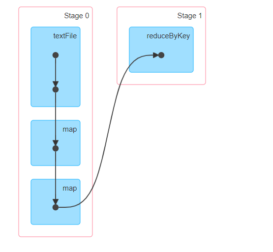
Drill into each stage, and you see that in the map phase, you will encounter shuffle write performance metrics in the map stage and shuffle read metrics in the reduce phase.
map phase =>

Reduce phase =>

So when someone asks you, “What are the benefits of Spark over Hadoop’s MR?”, do not answer with “spark uses another mechanism which replaces map-reduce”, because this is not true.
The correct answer is that spark has a very efficient Map-Reduce implementation, using in-memory computation at a distributed scale and this is what we are going to talk about here.
Iterative Algorithms
In big-data we will use iterative algorithms for:
- Approximations
When producing an accurate result required exponential complexity, we may opt to run approximated algorithms.
Some of these algorithms are iterative and the number of iterations determines the level of output accuracy. - Computation limits
For example, think about how social media platforms provide you with connection degrees.
Telling you if someone is your friend is simple, what about a friend of a friend? or friend of friend of friend?
Under the covers, each level requires another iteration of similar computation. - Iterative Machine Learning
Each iteration run strengthens our confidence in our prediction, many algorithms require multiple runs until reaching the desired error rate.
Also, in graph processing, iterative methods are quite common.
Iterative BFS – Breadth-First Search
Given a list of acyclic connection list, kept in the following CSV file, we would like to find the connection degrees of John to all other people in that list.
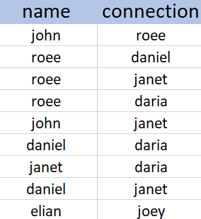
If we draw the graph of connections, we can easily mark each node with the correct connection degree to each user appearing in the file.
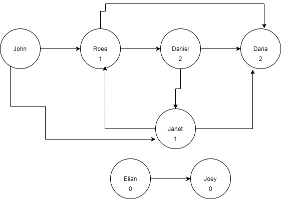
One solution would be to apply the BFS algorithm, where John is at the root
You can view a simulation with an explanation on BFS created by HackerEarth here
https://www.hackerearth.com/practice/algorithms/graphs/breadth-first-search/visualize/
Pseudo Algorithm
- q <- [john]
- connection_levels = []
- level = 1
- while q is not empty
- node <- q.pull()
- for all edge in edges.getEdgesFromSource (node)
- connection <- edge.destination()
- if connection_levels[connection] is not defined
- connection_levels[connection] = level
- q.push(connection)
Map Reduce
Let’s think about it on a big data scale. We need to think about how to represent that queue and the connections level map to be distributed.
What basically do these collections provide us?
- q- which connections are next to be examined
- connection_levels – which connections have already been examined
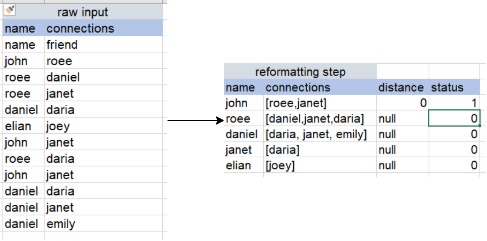
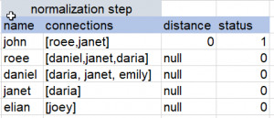
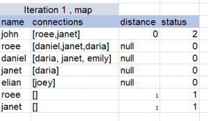
Consider the following representation for each node
(node, direct_connections, distant_from_source, status)
and we will initialize distant_from_source with null and status with ‘PENDING’, except for the initial node, where we will set RUNNING.
In our example,
- (john , [roee,janet] , 0, RUNNING)
- (roee, [daniel,daria, janet], null, PENDING)
- (daniel, [daria,janet], null , PENDING)
- (janet, [daria] , null , PENDING)
- (eilan, [joey], null, PENDING)
Let’s say we have 2 HDFS data nodes and not all connections’ edges are persisted to the same instance.
for example:
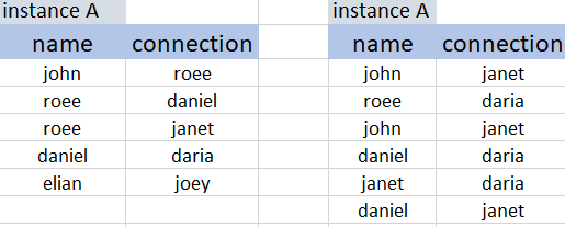
Filter
we start with only the records which are defined as ‘RUNNING’
Reduce
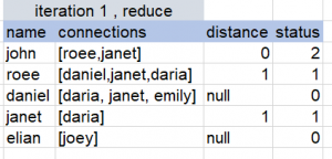
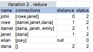
The reduce process will group the records by name, and transform the grouped list of (connections, distant, status) tuples to => (merge(connections), min (distances), max(status))
Once we have completed all these steps, we have basically accessed and marked all names with the distance of 1 from John.
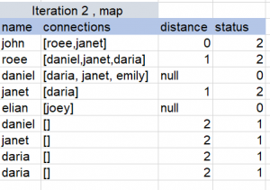
So we will have to repeat the map-reduce multiple times, you can view the following example to get a better understanding:
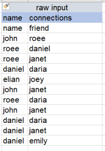
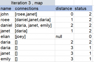
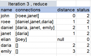
Iterative Algorithms in Hadoop
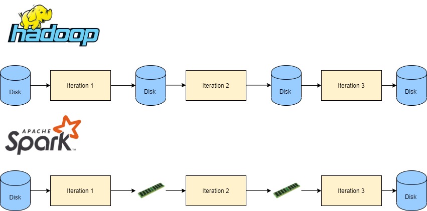
One important thing to remember about Hadoop is that it was first introduced in times where RAM memory was extremely expensive compared to these days, so it relies heavily on disk’s performance.
For the BFS algorithm we presented, what would happen is that Hadoop’s MR will store the result of each iteration in HDFS, and the following iteration will fetch that result as its input, so each iteration reads and writes from disk.
Iterative Algorithms in Spark
Spark introduces in-memory computation on a distributed scale, therefore it is highly efficient for iterative algorithms such as this because it places intermediate results in memory, which is the key difference between its implementation of map-reduce to what Hadoop’s MR offers.
Spark’s implementation
Before I summarize, I would like to show you the implementation.
note that we are going to do this in Kotlin, but don’t worry, you will still be able to understand the code if you are familiar with languages such as Java, Python, Scala.
If you would like to import the entire source code and run it on your local environment, it is available for you in this repository https://github.com/rzilkha/Bfs
Step 1 reading the file into a data frame
val fileName = args[0]
val source = args[1]
val iterations = Integer.valueOf(args[2])
val sparkSession = SparkSession.builder().appName("BFS")
    .orCreate
val dataframe = sparkSession.read()
    .option("header", true)
    .csv(fileName)
Step 2 – group connections by username
var data = dataframe.select(col("name"), col("connection"))
    .groupBy(col("name"))
    .agg(collect_set(col("connection")).`as`("connections"))
    .withColumn(
        "distance",
        ifElseColumn("name", source, 0, null)
    )
    .withColumn(
        "status",
        ifElseColumn("name", source, READY, PENDING)
    )
Iterations steps
help method – if-else column generator, used to make the code cleaner.. 🙂
fun ifElseColumn(column: String, compareValue: Any, value: Any?, elseValue: Any?): Column {
    return `when`(col(column).equalTo(compareValue), value ?: lit(null))
        .otherwise(elseValue ?: lit(null))
}
Step 1 -

1. create rows with the current distance for every connection in ready rows
2. set all previously “ready” rows to “done” state
=> adding these 2 steps together , will cause
here we will use a flatmap method to do both together
val schema: StructType? = StructType()
    .add(StructField.apply("name", DataTypes.StringType, true, null))
    .add(StructField.apply("connections", ArrayType.apply(DataTypes.StringType), true, null))
    .add(StructField.apply("distance", DataTypes.IntegerType, true, null))
    .add(StructField.apply("status", DataTypes.IntegerType, true, null))
fun explodeConnections(iteration: Int): (Row) -> Iterator {
    return {
        val name = it.getString(0)
        val connections = it.getList(1)
        val distance = it.get(2)
        val status = it.getInt(3)
        val normalized = mutableListOf()
        if (status == READY) {
            for (connection in connections) {
                normalized.add(RowFactory.create(connection, arrayOf(), iteration, READY))
            }
            normalized.add(RowFactory.create(name, connections.toTypedArray(), distance, DONE))
        } else {
            normalized.add(it)
        }
        normalized.iterator()
    }
}
and within each iteration, we will call:
data = data.flatMap(explodeConnections(i), rowEncoder)
Step 2 - reduce
data = data.select("*").groupBy(col("name"))
    .agg(
        flatten(collect_set(col("connections"))).`as`("connections"),
        min(col("distance")).`as`("distance"),
        max(col("status")).`as`("status")
    )
After iterations – Write to another csv file
data.select("name","distance").where(col("distance").isNotNull)
    .write()
    .mode("overwrite")
    .csv("output.csv")
Stages Graph
After running the task, let’s examine Spark’s monitoring after 3 iterations
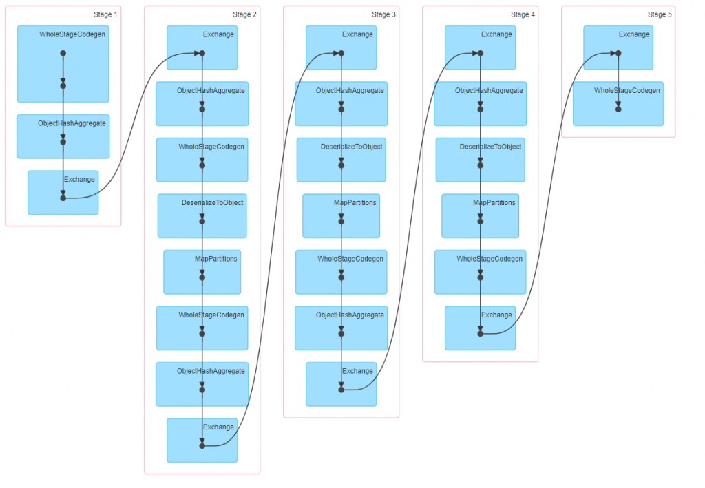 Here we see 5 Stages, and if I drill-down in to them, I can make up the logic each of them runs :
Stage 1 – is the preparation of the initial data prior to the iterative process:
- reading the CSV file,
- changing the dataframe’s schema to (name,[connections], distance, status]
Stage 2,3,4 – Each stage here is basically a map-reduce iteration
Stage 5 – last step, writing to a sink source, in our case, CSV file
Each Stage within a spark job contains multiple tasks, each computation its own partition, though in our specific context what’s interesting to know that between 2 stages there is a shuffle of data between one stage to the next.
What would be the Hadoop way to do that?
Here each iteration represents a single MR and you would need to write a mapper and a Reducer, which will run multiple times(3 in our case).
The mapper writes its result to disk, the reducers then fetch their relevant inputs files from HDFS and write the aggregated output to HDFS.
So if we run N iterations, then the number of disk reads/writes that occur between iterations is 2*N.
Comparing Spark and Hadoop
To conclude, Hadoop’s MR requires reading twice from disk in each iteration, once for reading the intermediate of the previous iteration and once for writing the iteration’s result for the next iteration, as its input.
Spark, on the other hand, enables transition between one iteration to the next without heavy disk reads/writes, as illustrated in this diagram
One thing to note here though, that it means nothing about what happens inside the iteration, map-shuffle-reduce phases still applies in both solutions, including disk usage, so the difference that we are focusing on here is between iterations only.
Nevertheless, there are also differences in how both technologies implement the shuffle phase and here to, Spark can optimize the process by being memory-intensive.
So to summarize:
- Spark is very efficient for iterative algorithms
- Spark replaces only Hadoop’s computation module, not the entire echo-system
- Spark also optimizes shuffles and other internal processes, but that is for another post.
